Two-Stage Object Detectors

Two stage object detectors Extracts feature from image and propose regions that likely contains objects and finally localize and classify these regions to detect object in the image.

Sliding Window Approach #

One method to detects the objects inside any image is to use sliding window approach. Here, we define boxes of different shapes and slide it over the image until we find the object.

This method is quite expensive as it have to generate boxes for each size and shape and need to run it through all the image.

But How about we just try only the regions that are interesting. i.e. Only reasons that may contain images?

That’s where Two stage object detectors come to play.

Region Proposals: #

• These proposes regions based on some interesting features such as same color pixels and so on.
• After obtaining region proposals, we just classify them whether the object lies in that box or not. If it does, we keep it, else remove it.

R-CNN (Region Convolutional Neural Networks) #

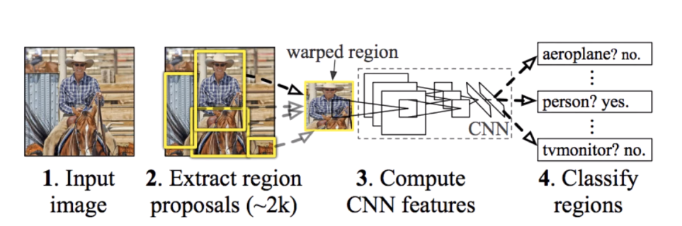
R-CNN takes region proposals and pass it to Convolution neural networks one by one to classify whether a object contains in that region or not, using Support Vector Machines.

Training Process:

1. Pre-Train the CNN on Image Net
2. Fine-tune the CNN on the number of classes the detector is aiming to classify (Softmax loss)
3. Train a support Linear Support machine classifier to classify image regions. One SVM per class (hinge loss)
4. Train the bounding box regressor (L2 loss)

Pros:

• Well Known method, so gives good results for detection and classification with SVM.
• Can be fine tuned for number of classes.

Cons

• Slow (takes 47s/image) with VGG16 backbone. one considers around 2000 proposals per image, they need to be wrapeds and forwarded through the CNN
• Training is slow

SPP Net #

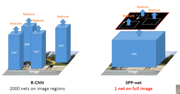
Takes all the regions at a time and classifies it and generated the bounding box unlike RCNN which takes one region at a time.

• Solved the R-CNN problem of being slow at test time

CONS

• Training was still slow
• Complex
• No end-to-end training. Separate training for feature extraction and

Histogram of Images #

count the number of pixels and plot accordingly. or group pixel numbers into bin of some size and count the number of pixels.

For RGB image, count colors of Red, Green and Blue channel separately.

Spatial Pyramid Matching #

While histograms give good knowledge about what colors and how much of these colors are present in the image, they cannot tell us about the visual similarity or dissimilarity.

As we can see in the below image, the histogram of both of the images will be same because both of the images contains the same amount of white and black pixels.

So, for that, we use Spatial Pyramid Matching.

In Spatial pyramid matching, we divide the image into numbers of grids and calculate the histogram of these grids separately.

This way, we get to know the colors present in eah section of image which gives us idea about visual differences between any images.

The final output of pyramid matching will be the concatenation of all these features. Let’s say we have a image of 8*8 pixels and we want 3 features from it. Then when we find the histogram and features of the image in 1x1 grid, it will be

$$ 3 \times 1 = 3 $$

Now, when we use $2 \times 2$ grid, we will have 3 features in each 4 grids so, it will be $3 \times 4 = 12$

Similarly for $4 \times 4$ grid it will be: $3 \times 16=48$ features.

Now, for the final output, we need to concatenate all of them, so the final concatenated output will be:

$$ 3 \times (1+4+16) $$

Which is,

$$ 3\times 21 $$

So, we can say here that the matching doesn’t depend on the size of image but on the features we are using.

Spatial Pyramid Pooling #

A paper SPPNet uses pyramid pooling as the last layer of AlexNet (in their paper) as a pyramid pooling layer. This method is similar to that of pyramid matching with some slight adjustments.

Here instead of creating histograms, codeblocks, they just max pool these grids. So, earlier, we were counting the features in each grid but now we just find maximum of that grid and use it as our final feature.

This way, the final output will be smaller than that in spatiial pyramid matching, as we can see in the below picture.

Now for image of depth 256 dimensions, the output will be $1\times256$, $4\times256$ and $16\times256$ which on concatenation becomes $21\times256$ dimensions feature vector.

Since, the Spatial Pooling is independent of image shape and size, we can use any size of image while training. Let’s say we have a image of $1000\times2000$ dimensions then we can just resize small size to someting smaller, assume $224$ then the largest size will be $448$. So, we can do this to other images and there won’t be any problem in training and testing.

But, cropping or warping the image to fixed size will reduce the accuracy of overall models.

SPP Net #

As we already know why the RCNN is slow in training and also in inference. When the region proposals gives us 2000 regions, we pass then one by one through feature extractor in the case of RCNN which becomes very slow in training and also in test time. But what will happen if we pass all the region proposals at the same time? It will be much faster isn’t it?

Yes it will.

And there comes our SPP Net. Here, we pass a single image to feature extractor and also to region proposal model. So, the feature extractor will be fast since it has to process only one image.

But,

But,

The training is still slow and complex

and we need to train separate models as it’s not end to end.

That’s where Fast-RCNN comes into play.

Fast R-CNN #

Fast RCNN takes out the region proposals layer and generates regions separately. Now the whole image is passed to conv net as in the SPPNet and region proposals also gets the whole image and generates 2000 regions.

Here, we apply ROI pooling to only those regions which are generated from region proposals after projecting them to the dimension that match the dimension of features extracted from feature extractor. This way we pass all the extracted region proposals at once and generate fixed sized feature vector from that which is passed to bounding box regressor and image classifier.

We can convert dynamic size image to fixed sized vectors since spatial pyramid pooling is independent of image shape and size and only depends on features. So, after pooling layer, we will be getting fixed sized vector even if the region proposals are of different shape and size which they will be.

Difference between SPPNet and Fast RCNN, here we can see that while SPPNet is using all the images when passing through pooling layer, Fast RCNN only takes specific regions to the pooling layer.

With ROI pooling the training time was increased by $8.8x$ than RCNN, the test time per image was increased by $146$ $\times$ ($0.32$ seconds for a image compared to 47 seconds in RCNN). Also increased mAP by 0.9 (66.9 vs 66.0). (2 seconds of image testing with region proposals)

But here the test time doesn’t include region proposal generation which if we include will be slower in inference.

So, to speed up the process Faster RCNN is introduced:

Faster R-CNN #

Problem statement:
Can we integrate a region proposal method inside neural network?
Now how can we design a network so that it can extract region proposals?

The only stand-alone portion of the network left in Fast R-CNN was the region proposal algorithm. Both R-CNN and Fast R-CNN use CPU based region proposal algorithms, Eg- the Selective search algorithm which takes around 2 seconds per image and runs on CPU computation. The Faster R-CNN paper fixes this by using another convolutional network (the RPN) to generate the region proposals. This not only brings down the region proposal time from 2s to 10ms per image but also allows the region proposal stage to share layers with the following detection stages, causing an overall improvement in feature representation.

Region Proposal Methods #

But, How many proposals do we need to generate, as we need some fixed number of proposals to genrate from neural networks.

Architecture #

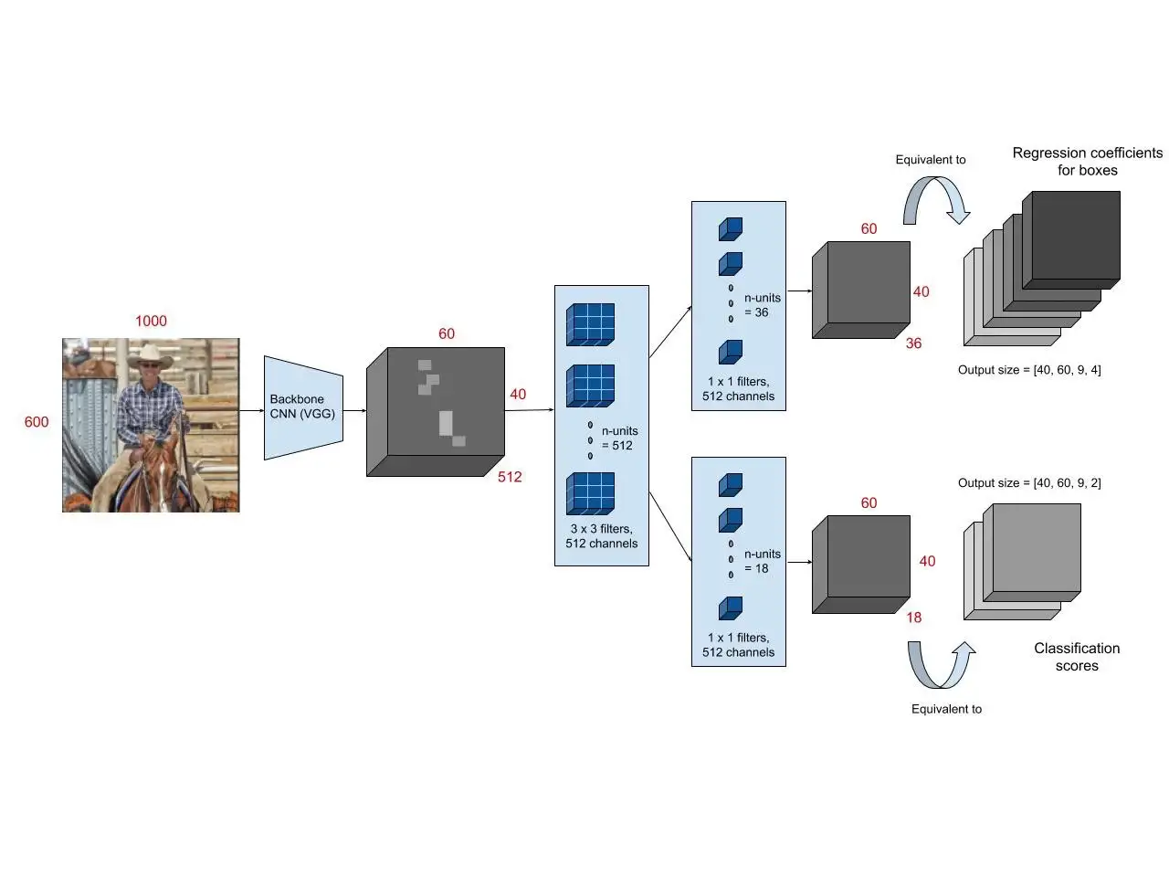
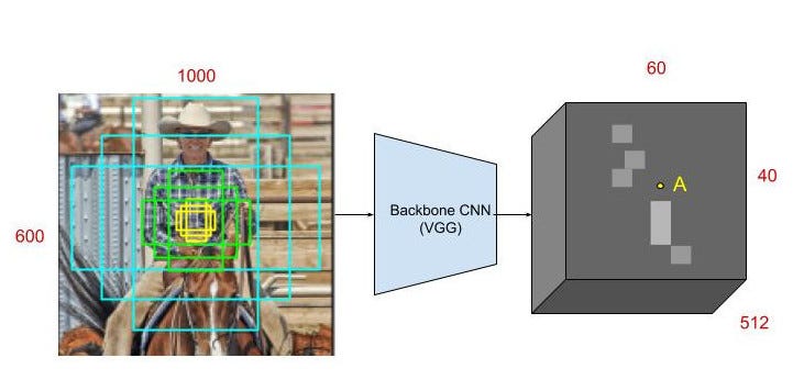
• The region proposal network (RPN) starts with the input image being fed into the backbone convolutional neural network. The input image is first resized such that it’s shortest side is 600px with the longer side not exceeding 1000px.
• The output features of the backbone network (indicated by H x W) are usually much smaller than the input image depending on the stride of the backbone network. For both the possible backbone networks used in the paper (VGG, ZF-Net) the network stride is 16. This means that two consecutive pixels in the backbone output features correspond to two points 16 pixels apart in the input image.
• For every point in the output feature map, the network has to learn whether an object is present in the input image at its corresponding location and estimate its size. This is done by placing a set of “Anchors” on the input image for each location on the output feature map from the backbone network. These anchors indicate possible objects in various sizes and aspect ratios at this location. The figure below shows 9 possible anchors in 3 different aspect ratios and 3 different sizes placed on the input image for a point A on the output feature map. For the PASCAL challenge, the anchors used have 3 scales of box area 128², 256², 512² and 3 aspect ratios of 1:1, 1:2 and 2:1.

• As the network moves through each pixel in the output feature map, it has to check whether these k corresponding anchors spanning the input image actually contain objects, and refine these anchors’ coordinates to give bounding boxes as “Object proposals” or regions of interest.
• First, a $3 \times 3$ convolution with 512 units is applied to the backbone feature map as shown in Figure, to give a $512d$ feature map for every location. This is followed by two sibling layers: a $1 \times 1$ convolution layer with 18 units for object classification, and a $1 \times 1$ convolution with 36 units for bounding box regression.
• The 18 units in the classification branch give an output of size $(H, W, 18)$. This output is used to give probabilities of whether or not each point in the backbone feature map (size: $H \times W$) contains an object within all 9 of the anchors at that point.
• The 36 units in the regression branch give an output of size $(H, W, 36)$. This output is used to give the 4 regression coefficients of each of the 9 anchors for every point in the backbone feature map (size: $H \times W$). These regression coefficients are used to improve the coordinates of the anchors that contain objects.

Training and Loss functions #

• The output feature map consists of about $40 \times 60$ locations, corresponding to $40\times60 \times9 \approx 20k$ anchors in total. At train time, all the anchors that cross the boundary are ignored so that they do not contribute to the loss. This leaves about 6k anchors per image.
• An anchor is considered to be a “positive” sample if it satisfies either of the two conditions — a) The anchor has the highest IoU (Intersection over Union, a measure of overlap) with a groundtruth box; b) The anchor has an IoU greater than 0.7 with any groundtruth box. The same groundtruth box can cause multiple anchors to be assigned positive labels.
• An anchor is labeled “negative” if its IoU with all groundtruth boxes is less than 0.3. The remaining anchors (neither positive nor negative) are disregarded for RPN training.
• Each mini-batch for training the RPN comes from a single image. Sampling all the anchors from this image would bias the learning process toward negative samples, and so 128 positive and 128 negative samples are randomly selected to form the batch, padding with additional negative samples if there are an insufficient number of positives.
• The training loss for the RPN is also a multi-task loss, given by:

$$L({p_i}, {t_i}) = \frac{1}{N_{cls}}\sum_iL_{cls}(p_i, p_i^\ast) + \lambda \frac{1}{N_{reg}}\sum_i p_i^\ast L_{reg}(t_i, t_i^\ast)$$

• Here $i$ is the index of the anchor in the mini-batch. The classification loss $L_{\text{cls}}(p, p_i)$ is the log loss over two classes (object vs not object). $p_i$ is the output score from the classification branch for anchor $i$, and $p_i$ is the groundtruth label (1 or 0).
• The regression loss $L_{reg}(t_i, t_i^\ast)$ is activated only if the anchor actually contains an object i.e., the groundtruth $p_i$ is $1$. The term $t_i$ is the output prediction of the regression layer and consists of 4 variables $[t_x, t_y, t_w, t_h]$. The regression target $t_i^\ast$ is calculated as —

$$t^\ast_x = \frac{x^\ast - x_a}{w_a} $$ $$t^\ast_y = \frac{y^\ast - y_a}{h_a} $$ $$t^\ast_w = \log{(\frac{h^\ast}{h_a})}$$

Here $x$, $y$, $w$, and $h$ correspond to the $(x, y)$ coordinates of the box centre and the height $h$ and width $w$ of the box.
$x_a$ and $x^*$ stand for the coordinates of the anchor box and its corresponding groundtruth bounding box.

• Remember that all k (= 9) of the anchor boxes have different regressors that do not share weights. So the regression loss for an anchor i is applied to its corresponding regressor (if it is a positive sample).
• At test time, the learned regression output tᵢ can be applied to its corresponding anchor box (that is predicted positive), and the x, y, w, h parameters for the predicted object proposal bounding box can be back-calculated from — $$t_x = \frac{x- x_a}{w_a}$$ $$t_y = \frac{y- y_a}{h_a}$$ $$t_w = \log{(\frac{w}{w_a})}$$ $$t_h = \log{(\frac{h}{h_a})}$$

Object detection: Faster R-CNN (RPN + Fast R-CNN) #

The Faster R-CNN architecture consists of the RPN as a region proposal algorithm and the Fast R-CNN as a detector network.

4 Step Alternating training #

In order to force the network to share the weights of the CNN backbone between the RPN and the detector, the authors use a 4 step training method:

1. The RPN is trained independently as described above. The backbone CNN for this task is initialized with weights from a network trained for an ImageNet classification task, and is then fine-tuned for the region proposal task.
2. The Fast R-CNN detector network is also trained independently. The backbone CNN for this task is initialized with weights from a network trained for an ImageNet classification task, and is then fine-tuned for the object detection task. The RPN weights are fixed and the proposals from the RPN are used to train the Faster R-CNN.
3. The RPN is now initialized with weights from this Faster R-CNN, and fine-tuned for the region proposal task. This time, weights in the common layers between the RPN and detector remain fixed, and only the layers unique to the RPN are fine-tuned. This is the final RPN.
4. Once again using the new RPN, the Fast R-CNN detector is fine-tuned. Again, only the layers unique to the detector network are fine-tuned and the common layer weights are fixed.

This gives a Faster R-CNN detection framework that has shared convolutional layers.

	R-CNN	Fast R-CNN	Faster R-CNN
Test time per img (with proposals)	$50$ seconds	$2$ seconds	$0.2$ seconds
Speedup	$1$x	$25$x	$250$x
mAP (VOC 2007)	$66.0$	$66.9$	$66.9$

References #

1. C 7.2 | Spatial Pyramid Matching | SPM | CNN | Object Detection | Machine learning | EvODN
2. C 7.3 | Spatial Pyramid Pooling | SPPNet Classification | Fast RCNN | Machine learning | EvODN
3. C 7.5 | ROI Projection | Subsampling ratio | SPPNet | Fast RCNN | CNN | Machine learning | EvODN
4. C 8.1 | Faster RCNN | Absolute vs Relative BBOX Regression | Anchor Boxes | CNN | Machine Learning
5. Faster R-CNN for object detection