Understanding Recurrent Neural Networks (RNNs) for Sequential Data Processing

Introduction #

You may have already worked with feedforward neural networks, these neural networks take input and after some computation in hidden layers they produce output. which works in most of the cases but when it comes with sequential data like text, sound, stock price we cannot just predict next value from only one previous inputs, we need some contexts to generate the next output which is impossible with feedforward neural networks.

What is sequential data? #

Sequential data is that type of data that comes in sequence. Consider we have a weather data. The weather of the next day depends not only on other factors but also on previous days’ weather too. So, the data that depends on previous data for future prediction is called sequential data. Text, Weather data, stock prices, audio data are the best example of sequential data.

So, let’s head back to RNNs, RNNs are that type of neural networks that can process these sequential data. They use memory cells to keep track of previous inputs in the form of hidden state and use it to compute the overall prediction of neural network.

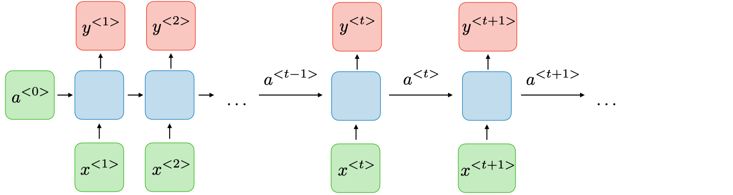
Here, we can see each RNN units returns two outputs, one hidden state that is passed to another RNN cell for next prediction and another prediction of that cell.

Here,

$x^{<t>}$ = input data of $t^{th}$ timestep

$a^{<t>}$ = hidden state of $t^{th}$ timestep

$y^{<t>}$ = output of $t^{th}$ timestep

Basically, the first input takes initial hidden state $a^{<0>}$ which we initialize randomly along with input $x^{<1>}$ which produces the output $y^{}$ using the following formula.

$$ a^{<1>} = g(W_{aa}a^{0} + W_{ax}X^{1} + b_a) $$

$$ \hat{y}^{<1>} = g’(W_{ya}a^{<1>} + b_y) $$

In general,

$$ a^{<t>} = g(W_{aa}a^{t-1} + W_{ax}X^{t} + b_a) $$

$$ \hat{y}^{<t>} = g’(W_{ya}a^{<t>} + b_y) $$

Where,

$W_{aa}$ is the weight vector of hidden state

$W_{ax}$ is the weight vector of input edge

$W_{ya}$ is the weight vector of output

$b_a$ is the bias term for hidden state

$b_y$ is the bias term for output

In each time-step, we use previous hidden state and current input to calculate the next output. Since RNNs share parameters across time, here we are using only two sets of weight vector for every time steps mainly for input state and hidden state. The output layer is just as same as the feedforward neural network.

The back-propagation operation is same as we do in feedforward neural networks but since we are using different time-steps, we average the gradients of every timestep to calculate the final output, and the we call this backpropagation, backpropagation through time.

Types of Recurrent Neural Networks #

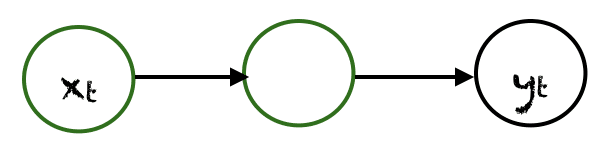
1. One to One

   In this type of RNNs there will be one input and one output.

   example:

   • Traditional Neural Networks

   

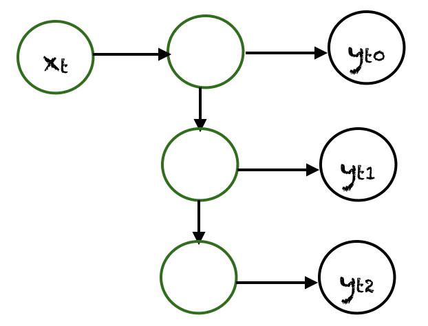
2. One to Many

   If there is only one input and many outputs then this type of RNN is called One to Many RNN. example:

   • generating music from a single tune or empty subset.

   

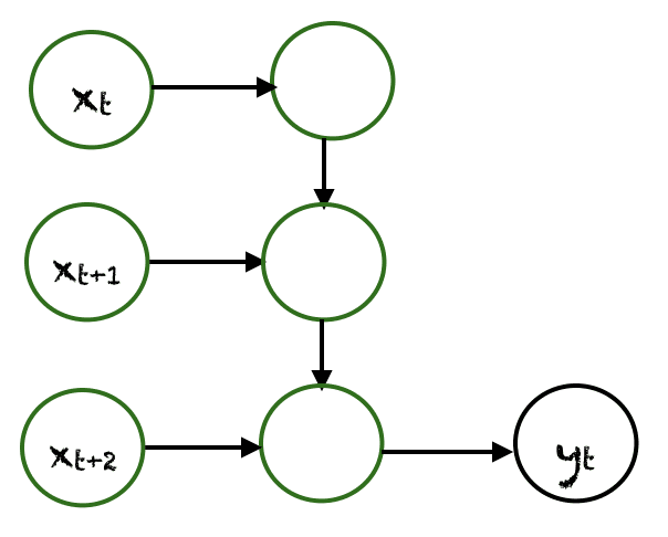
3. Many to One

   When there are multiple inputs but the output is only one, then this type of RNN is called many to one RNN.

   example:

   • Calculating sentiment from long text.
   • Classifying news articles to different categories.

   

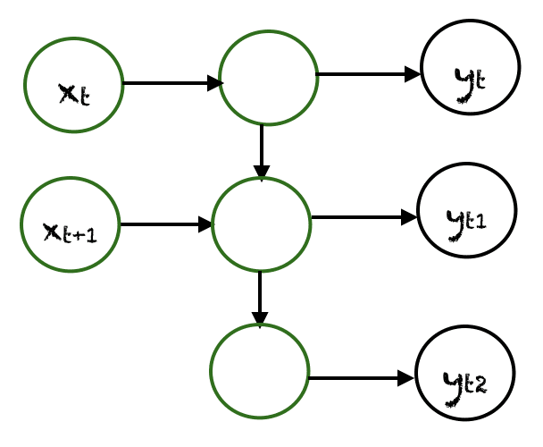
4. Many to Many

   If there are many inputs and many outputs then this type of RNN is called Many to Many architecture.

   example:

   • Text generation
   • Language Translation

   

Cons of RNNs #

Vanishing Gradients #

While RNNs works best with sequential data, they struggle with large sequences. If we have long sequence of text and we need to generate text based on that, we need to have context of the words present in beginning of sentence to correctly predict the word in the next sequence, but since it cannot hold a lot of information, there will be almost no impact of these words in the sequence. This type of problem is called vanishing gradients.

Mathematically, If the sequence is too large and the weights becomes less than 1 then the impact of words which are far before current words will be low while predicting current word and the prediction may become wrong.

Exploding Gradients #

If the weights of RNN > 1 then the weights may increase exponentially in every iteration and can cause numerical overflow.

We can reduce exploding gradients problem using gradient clipping.