Demystifying Quantization: Shrinking Models for Efficient AI

Quantizaton Representative image (stablediffusionweb.com)

Introduction #

Large Language Models (LLMs) are revolutionizing AI research these days. Many tasks that once required complex models can now be solved in minutes with the help of LLMs. Not only are they generation models, but they can also tackle summarization, classification, question answering, clustering, and much more. While all these benefits are fantastic, using LLMs on your own machine can be challenging due to their size. Most LLMs require larger GPUs to run, which might be feasible for big companies but can be a stumbling block for individuals.

Enter quantization. Quantization is a method that significantly reduces the size of any model. In quantization, we convert the model’s parameters from higher precision, like FLOAT32 (FP32), to lower precision, such as INT4 or INT8. This greatly shrinks the model’s size. However, since we’re reducing the precision of the model’s parameters, there’s a slight decrease in accuracy. But the trade-off in size might be well worth it.

But, why do we need Quantization? #

As I mentioned earlier, running an LLM with 100 billion parameters on your computer is not feasible, so we need a way to run these models on our machines without significant performance degradation. Models are usually trained in higher precision, i.e., FLOAT32, and when we quantize these models, we typically convert them to a lower precision range like INT8 or even INT4.

Let’s use an LLM as an example. Llama3-70B has 70 billion parameters. To store this model in full precision, i.e., FP32, we need $70 \space billion \times 32 \space bit = \frac{70 \times 10^9 \times 32}{8 \times 10^9} = 280 \space GB$ of storage.

Now, let’s also calculate the GPU memory (VRAM) required to run this 70 billion parameter model.

We have a formula.

$$ Memory \space required (M) \approx \frac{P \times 4 \space bytes}{ \frac{32}{Q} } \times 1.2 $$ $$\text{or} $$ $$\frac{P \times Q \times 4 \space bytes}{32} \times 1.2$$

$Where$,

Symbol	Description
$ M $	GPU memory expressed in Gigabyte
$P$	The amount of parameters in the model. E.g. a 7B model has 7 billion parameters.
$4 \space bytes$	4 bytes, expressing the bytes used for each parameter
$32$	There are 32 bits in 4 bytes
$Q$	The amount of bits that should be used for loading the model. E.g. 16 bits, 8 bits or 4 bits.
$1.2$	Represents a 20% overhead of loading additional things in GPU memory.

$$ M \approx \frac{70 \times 4 \times 32}{32} \times 1.2 = 336 \space GB $$

So, the memory required to run the LLama3-70B in full precision is approximately 336 GB.

This is really high, since we need high end GPU or multiple GPUs to run this model in full precision. Even if we take smaller models like 7B or 8B, we need almost 28 GB VRAM.

This seems impossible for individual users. But if we quantize the same model in 4-bit or 8-bit we need much smaller VRAM. let’s calculate:

For 4-bit $$ M \approx \frac{7 \times 4 \times 4}{32} \times 1.2 $$ $$M \approx 4.2 \space GB$$

For 8-bit $$ M \approx \frac{7 \times 8 \times 4}{32} \times 1.2 $$ $$M \approx 8.4 \space GB$$

Even after quantization, these models require much larger GPU RAM. But these are in acceptable range as we can run these models simply in our computer.

So, quantization helps us use these models on smaller GPU without much performance degradation.

How Computer Stores Numbers #

Before delving into the details of how we quantize models from high precision to low precision, let’s take a look at how computers store numbers in CPU or memory. For every bit of a number, the computer requires an equal amount of storage. For instance, if we have a 32-bit number, the computer will use 32 bits to store that number in memory.

Computers store numbers in two ways: Unsigned and Signed. A Signed value will store the sign (positive or negative) of the number, while an Unsigned value cannot store the sign of the number. To store the sign of any number, the computer uses 1 bit of memory.

Let’s look an example on how a 8-bit Unsigned integer stored in memory.

$1$	$0$	$0$	$0$	$1$	$0$	$0$	$1$

$2^7 \quad+ \quad 0 \quad+\quad 0 \quad+\quad 0 \quad+ \quad 2^3 \quad+ \quad0 \quad+ \quad0\quad +\quad 2^0\quad = \quad 137$

The range of integers an 8-bit integer can store is calculated as: $range \space [0, 2^n-1] = [0, 255] $ for 8-bit unsisigned integers. This means that, it can only stores values from 0 to 255. If the value lies beside these boundaries, then they will be set as either 0 for smaller and 255 for larger value.

This is different for signed integers, as the range is calculated as: $$range \space [- \space 2^{n-1}, 2^{n-1}-1]$$

For 8-bit signed integers the range will be $[-128, 127]$

This is completely different when it comes to floating point numbers. In floating point numbers, we will have three components:

Sign
Exponent or Range
Fraction or Precision or Mantissa

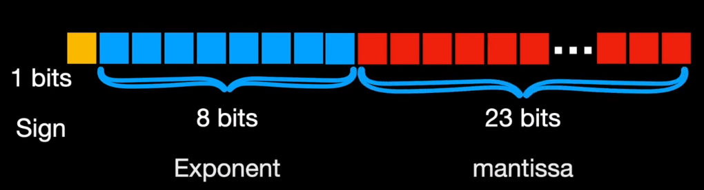
Below, you can see how computer stores floating point numbers. Each of these formats consume different chunk of the memory. For example, float32 allocates 1 bit for sign, 8 bits for exponent and 23 bits for mantissa.

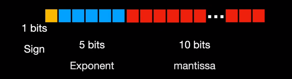
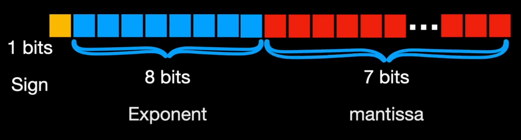
Similarly, float16 or FP16 allocates 1 bit for sign but just 5 bits for exponent and 10 bits for mantissa. On the other hand, BF16 (B stands for Google Brain) allocates 8 bits for the exponent and just 7 bits for mantissa.

So, in short the conversion from a higher memory format to a lower memory format is called quantization. Talking in deep learning terms, Float32 is referred to as single or full precision and Float16 and BFloat16 are called half precision. The default way in which deep learning models are trained and stored is in full precision. The most commonly used conversion is from full precision to an int8 and int4 format.

Types of Quantization #

When considering the types of quantization available for use during model compression, there are 2 main types to pick from

Asymmetric Quantization #

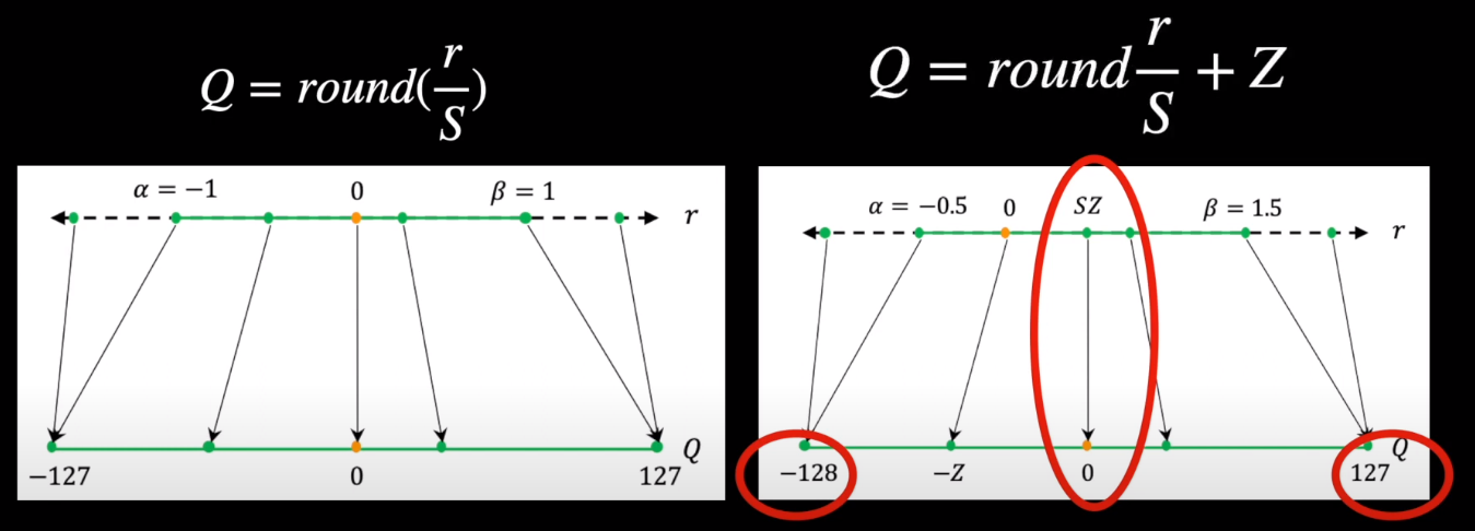
In asymmetric mode, we map min-max of dequantized value to min-max range of target precision. This is done by using zero-point also called quantization bias. Here zero point can be non-zero value.

$$X_q = clamp \left( \frac{X}{S} + Z ; 0, 2^n - 1\right)$$ Where, $$ clamp(x;a,c) = \begin{cases} a &\quad x < a \\ x &\quad a \le x \le c \\ c &\quad x>c \end{cases} $$

$$ S = \frac{X_{max} - X_{min}}{2^n - 1} $$

$$Z = -\frac{X_{min}}{S}$$

Here,

$X \quad = $ Original floating point tensor
$X_q \quad = $ Quantized Tensor
$S \quad=$ Scale Factor
$Z \quad= $ Zero Point
$n \quad= $ Number of bits used for quantization

Note that in the derivation above we use unsigned integer to represent the quantized range. That is, $X_q∈[0,2^n−1]$. One could use signed integer if necessary (perhaps due to HW considerations). This can be achieved by subtracting $2^n−1$ .

Python Implementation #

Now let’s implement Asymmetric quantization in python.

First, we import the required library. We are using pytorch here.

import torch

_ = torch.random.manual_seed(1)

Now, let’s define the required functions:

def clamp(X:torch.Tensor, val_range:tuple):
    """Clamps the Tensor between given range"""
    min_range, max_range = val_range
    # X[X < min_range] = min_range
    # X[X> max_range] = max_range
    return torch.clip(X, min_range, max_range)
    
def scale(X, target_bits):
    X_max = torch.max(X)
    X_min = torch.min(X)
    return (X_max - X_min) / (2^target_bits - 1)

def zero_point(X, S):
    return - torch.round(torch.min(X)/ S)


def quantize(X, target_bits):
    S = scale(X, target_bits)
    Z = zero_point(X, S)
    X_q = torch.round((X/S) + Z)
    X_q = clamp(X_q, (0, 2^target_bits - 1)) 
    #  Range will be (-2^target_bits-1, 2^target_bits - 1) if we use signed integer
    torch_dype_map = {
        8: torch.int8,
        16: torch.int16,
        32: torch.int32
    }
    dtype = torch_dype_map[target_bits]
    return X_q.to(dtype), S, Z

def dequantize(X_q, S, Z):
    return S * (X_q - Z)

def quantization_error(X, X_dequant):
    return torch.mean((X- X_dequant)**2)

Now, Let’s See the results. We inititlilze a random tensor of size (5,5) and check the quantization error.

# Let's inititalize a random tensor of size (5,5) between -127 and 127
X = torch.FloatTensor(5, 5).uniform_(-127, 127)
print("The original Tensor is: ")
print(X)
# Quantization
X_q, S, Z = quantize(X, 8)

print("After Quantization:")
print(X_q)
print(f"Scale factor: {S}, Zero Point: {Z}")

print("After Dequantization: ")
X_dequant = dequantize(X_q, S, Z)
print(X_dequant)

q_mse = quantization_error(X, X_dequant)
print(f"Quantization Error: {q_mse}")

OUTPUT:

The original Tensor is: 
tensor([[ -64.7480,   89.2118,    0.8170, -101.9451,  -26.6123],
        [-114.6317,  -65.7990,  -89.9714,   86.8619,  -26.6812],
        [ -21.9427,   60.8604,   51.6853,  -83.8159,   46.8039],
        [  53.9525, -100.9789,  110.4185,  -77.2771,  -49.6635],
        [-104.6081,  116.0752,   24.1830,  106.9384,    8.2932]])
tensor([[1., 4., 2., -0., 1.],
        [-0., 1., 0., 4., 1.],
        [2., 3., 3., 0., 3.],
        [3., -0., 4., 0., 1.],
        [-0., 5., 3., 4., 2.]])
After Quantization:
tensor([[1, 4, 2, 0, 1],
        [0, 1, 0, 4, 1],
        [2, 3, 3, 0, 3],
        [3, 0, 4, 0, 1],
        [0, 5, 3, 4, 2]], dtype=torch.int8)
Scale factor: 46.141387939453125, Zero Point: 2.0
After Dequantization: 
tensor([[-46.1414,  92.2828,   0.0000, -92.2828, -46.1414],
        [-92.2828, -46.1414, -92.2828,  92.2828, -46.1414],
        [  0.0000,  46.1414,  46.1414, -92.2828,  46.1414],
        [ 46.1414, -92.2828,  92.2828, -92.2828, -46.1414],
        [-92.2828, 138.4242,  46.1414,  92.2828,   0.0000]])
Quantization Error: 202.06419372558594

As, we can see there is quite the data loss when quantizing the tensor with Mean Squared error 202.06, which is really high. But we have more optimized methods these days, so the data loss will be really small. Also, see how the tensor performs when we dequantize it, we can see huge difference there also.

Symmetric Quantization #

In symmetric quantization when converting from higher precision to lower precision, we can always restrict to values between $[-(2^{n-1} - 1), \space + 2^{n-1}-1]$ and ensure that the zero of the input perfectly maps to the zero of the output leading to a symmetric mapping. For FLOAT16 to INT8 Conversion, we restrict the values between -127 to +127.

Here, $$X_q = clamp \left( \frac{X}{S} ; - (2^{n-1} -1), (2^{n-1} - 1)\right)$$ Where, $$ S = \frac{ |X|_{max}}{2^{n-1} - 1} $$

$$Z = 0$$

Python Implementation #

import torch
_ = torch.random.manual_seed(1)

def clamp(X:torch.Tensor, val_range:tuple):
    """Clamps the Tensor between given range"""
    min_range, max_range = val_range
    # X[X < min_range] = min_range
    # X[X> max_range] = max_range
    return torch.clip(X, min_range, max_range)
    

def scale(X, target_bits):
    X_max = torch.max(torch.abs(X))
    return (X_max) / (2^(target_bits-1) - 1)


def quantize(X, target_bits):
    S = scale(X, target_bits)
    X_q = torch.round(X/S)
    X_q = clamp(X_q, (-2^(target_bits-1) - 1, 2^(target_bits-1)-1))
    torch_dype_map = {
        8: torch.int8,
        16: torch.int16,
        32: torch.int32
    }
    dtype = torch_dype_map[target_bits]
    return X_q.to(dtype), S

def dequantize(X_q, S):
    return S * X_q

def quantization_error(X, X_dequant):
    return torch.mean((X- X_dequant)**2)


# Let's inititalize a random tensor of size (5,5) between -127 and 127
X = torch.FloatTensor(5, 5).uniform_(-127, 127)
print("The original Tensor is: ")
print(X)
# Quantization
X_q, S = quantize(X, 8)

print("After Quantization:")
print(X_q)
print(f"Scale factor: {S}")

print("After Dequantization: ")
X_dequant = dequantize(X_q, S)
print(X_dequant)

q_mse = quantization_error(X, X_dequant)
print(f"Quantization Error: {q_mse}")

OUTPUT:

The original Tensor is: 
tensor([[   6.0810,   75.7082,   69.0292, -124.1490,   78.7299],
        [  35.4792,  120.4665,   83.8276, -115.7145, -120.7527],
        [ -61.2562,  111.5202,  -21.1543,   54.3508,  -59.0183],
        [ 124.6147,  -53.7335,   95.2404,    1.5039,  -66.9058],
        [  65.2799,  -67.4142,   37.3513,  -36.6722,  -13.9236]])
After Quantization:
tensor([[ 0,  2,  2, -4,  3],
        [ 1,  4,  3, -4, -4],
        [-2,  4, -1,  2, -2],
        [ 4, -2,  3,  0, -2],
        [ 2, -2,  1, -1,  0]], dtype=torch.int8)
Scale factor: 31.153671264648438
After Dequantization: 
tensor([[   0.0000,   62.3073,   62.3073, -124.6147,   93.4610],
        [  31.1537,  124.6147,   93.4610, -124.6147, -124.6147],
        [ -62.3073,  124.6147,  -31.1537,   62.3073,  -62.3073],
        [ 124.6147,  -62.3073,   93.4610,    0.0000,  -62.3073],
        [  62.3073,  -62.3073,   31.1537,  -31.1537,    0.0000]])
Quantization Error: 57.84915542602539

BUT, Which method is better? #

Asymmetric range fully utilizes the quantized range because we exactly map the min-max values from float to the min-max range of quantized range. While in Symmetric, if the float range is biased towards one side, it could result in a quantized range where significant dynamic range is dedicated to values that we’ll never see. This could result in greater loss.
Also Zero point in asymmetric quantization leads extra weight on Hardware as it requires extra calculation, while the symmetric quantization is much simpler when we compare it to asymmetric. So we mostly use symmetric quantization.

Choosing Scale Factor and Zero point #

Above, we saw that the zero point of symmetric quantization is zero, while it is different in case of Asymmetric quantization. How do we decide this? Let’s take an example, Every integer or floating point number will have their own range (-128 to 127 for int8), the scaling factor essentially divides these numbers into equal factor. Since, when quantization, the high precision values should be reduced to lower precision, we need to clip those values at some point say alpha and beta for negative and positive values respectively. Any value beyond alpha and beta is not meaningful because it maps to the same output as that of alpha and beta. For the case of INT8 its -127 and +127 (we use -127 or numerical stability, this is called restricted quantization). The process of choosing these clipping values alpha and beta and hence the clipping range is called calibration.

To avoid cutting off too many numbers, a simple solution is to set alpha to $X_{\text{min}}$ and beta to $X_{\text{max}}$. Then we can easily figure out the scale factor, $S$, using these smallest and largest numbers. But this might make our counting uneven. For instance, if the largest number ($X_{\text{max}}$) is 1.5 and the smallest ($X_{\text{min}}$) is -1.2, our counting isn’t balanced. To make it fair, we pick the larger number between the two ends and use that as our cutoff point on both sides. And we start counting from 0.

This balanced counting method is what we use when simplifying neural network weights. It’s simpler because we always start counting from 0, making the math easier.

Now, let’s consider when our numbers are mostly on one side, like the positive side. This is similar to the outputs of popular activation functions like ReLU or GeLU. Also, these activation outputs change based on the input. For example, showing the network two images of a cat might give different outputs. ¹

While, Minimum and maximum value works, sometimes we may see outliers that affect in quantization, in such cases, we can choose percentiles to choose the value of alpha and beta.

Modes of Quantization #

Based on when to quantize the model weights, quantization can be thought as two modes:

1. Post-Training Quantization (PTQ) #

In Post-Training quantization or PTQ, we quantize the weights of already trained model. This is straightforward and easy to implement, however it may degred the performance of model slightly due to the loss of precision in the value of weights.
To better calibrate the model, model’s weight and activations are evaluated on a representative dataset to determine the range of values (alpha, beta, scale, and zero-point) taken by these parameters. We then use these parameters to quantize the model.

Based on the methods of quantization, we can further divide PTQ into three categories:

Dynamic-Range Quantization: In this method, quantize the model based on the range of data globally. This method produces small model but there may be a bit more accuracy loss.
Weight Quantization: In this method, we only quantize the weights of model leaving activations in their high precision. There may be higher accuracy loss with this method.
Per-Channel Quantization: In this method, we quantize the model parameters based on the dynamic range per channel rather than globally. This helps in achieving optimal accuracy.

Implementation using PyTorch #

Import all the necessary libraries

import os
from tqdm import tqdm

import torch
import torch.nn as nn
import torchvision.datasets as datasets
import torchvision.transforms as transforms

_ = torch.manual_seed(0)

Download and load the dataset:

transform = transforms.Compose([transforms.ToTensor(), transforms.Normalize((0.1301, ), (0.3081, ))])

mnist_trainset = datasets.MNIST(root = "./data", train = True, download=True, transform=transform)

train_loader = torch.utils.data.DataLoader(mnist_trainset, batch_size=10, shuffle=True)

mnist_testset = datasets.MNIST(root = "./data", train=False, download=True, transform=transform)
test_loader = torch.utils.data.DataLoader(mnist_testset, batch_size=10)

device = torch.device("cpu")

Create a simple pytorch model.

class DigitsNet(nn.Module):
    def __init__(self, input_shape, num_classes):
        super(DigitsNet, self).__init__()
        self.linear1 = nn.Linear(input_shape, 100)
        self.linear2 = nn.Linear(100, 100)
        self.linear3 = nn.Linear(100,num_classes)
        self.relu = nn.ReLU()

    def forward(self, x):
        x = self.linear1(x)
        x = self.linear2(x)
        x = self.linear3(x)
        x = self.relu(x)
        return x
    
model = DigitsNet(28*28, 10).to(device)

Now, let’s create a simple training loop to train and test the model

def train(train_loader, model, epochs = 5, limit=None):
    ce_loss = nn.CrossEntropyLoss()
    optimizer = torch.optim.Adam(model.parameters(), lr=0.001)

    total_iterations = 0
    for epoch in range(epochs):
        model.train()
        loss_sum = 0
        num_iterations = 0
        data_iterator = tqdm(train_loader, desc=f"Epoch {epoch+1}")

        if limit is not None:
            data_iterator.total = limit
        
        for data in data_iterator:
            num_iterations += 1
            total_iterations += 1
            x, y = data
            x = x.to(device)
            y = y.to(device)

            optimizer.zero_grad()
            output = model(x.view(-1, 28*28))
            loss = ce_loss(output, y)
            loss_sum += loss
            avg_loss = loss_sum / num_iterations
            data_iterator.set_postfix(loss=avg_loss.item())
            loss.backward()
            optimizer.step()

            if limit is not None and total_iterations >= limit:
                return

def test(model):
    correct = 0
    total = 0
    wrong_counts = [0 for i in range(10)]

    with torch.no_grad():
        for data in tqdm(test_loader, desc="Testing"):
            x, y = data
            x = x.to(device)
            y = y.to(device)
            output= model(x.view(-1, 28*28))
            for idx, i in enumerate(output):
                if torch.argmax(i) == y[idx]:
                    correct += 1
                else:
                    wrong_counts[y[idx]] += 1
                total+=1
        print(f"Accuracy: {round(correct/total, 3) * 100}")

Create a function to see the model size.

def print_model_size(model):
    torch.save(model.state_dict(), "temp_model.pt")
    print("Size (KB): ", os.path.getsize("temp_model.pt")/1e3)
    os.remove("temp_model.pt")

Now, Let’s train the model for 1 epochs.

train(train_loader, model, epochs=1)

Epoch 1: 100%|██████████| 6000/6000 [00:12<00:00, 488.88it/s, loss=0.651]

Before quantizing the model, let’s check the weight of a layer.

# weights before quantization
print(model.linear1.weight)
print(model.linear1.weight.dtype)

Parameter containing:
tensor([[-0.0267, -0.0073, -0.0558,  ..., -0.0045, -0.0227, -0.0243],
        [-0.0445, -0.0397, -0.0352,  ..., -0.0450, -0.0307, -0.0547],
        [-0.0326,  0.0025, -0.0457,  ..., -0.0328, -0.0113, -0.0044],
        ...,
        [ 0.0179,  0.0216, -0.0130,  ..., -0.0184,  0.0009, -0.0361],
        [-0.0138, -0.0057,  0.0264,  ...,  0.0067,  0.0067,  0.0062],
        [ 0.0057,  0.0003, -0.0138,  ...,  0.0226, -0.0267, -0.0065]],
       requires_grad=True)
torch.float32

As we can see our original weights are in float32. Also, Let’s check the size and accuracy of the model

# size of model
print_model_size(model)

# accuracy
test(model)

Size (KB):  360.998
Testing: 100%|██████████| 1000/1000 [00:00<00:00, 1746.29it/s]
Accuracy: 90.60000000000001

Our original model size before quantizing is 360KB with 90.6% accuracy. Now let’s quantize the model.

To quantize the model, we first create a exact copy of model with two extra layers, i.e. quant and dequant. These layers basically help us in finding the optimal range.

class QuantizedDigitsNet(nn.Module):
    def __init__(self, input_shape, num_classes):
        super(QuantizedDigitsNet, self).__init__()
        self.quant = torch.quantization.QuantStub()
        self.linear1 = nn.Linear(input_shape, 100)
        self.linear2 = nn.Linear(100, 100)
        self.linear3 = nn.Linear(100,num_classes)
        self.relu = nn.ReLU()
        self.dequant = torch.quantization.DeQuantStub()

    def forward(self, x):
        x = x.view(-1, 28*28)
        x = self.quant(x)
        x = self.linear1(x)
        x = self.linear2(x)
        x = self.linear3(x)
        x = self.relu(x)
        x = self.dequant(x)
        return x

As I said earlier, we introduce model with some test set to calibrate the range. This gives us idea about the values of $\alpha$, $\beta$, $S$ and $Z$. In above model, we used two observers to observe the model behaviour. These observers calculate the required values when we calibrate the model. To calbrate it we simply pass the test set to dataset for a epoch.


# calibration

import torch.ao.quantization


model_quantized = QuantizedDigitsNet(28*28, 10).to(device)

model_quantized.load_state_dict(model.state_dict())
model_quantized.eval()

model_quantized.qconfig = torch.ao.quantization.default_qconfig
model_quantized = torch.ao.quantization.prepare(model_quantized)
model_quantized

QuantizedDigitsNet(
  (quant): QuantStub(
    (activation_post_process): MinMaxObserver(min_val=inf, max_val=-inf)
  )
  (linear1): Linear(
    in_features=784, out_features=100, bias=True
    (activation_post_process): MinMaxObserver(min_val=inf, max_val=-inf)
  )
  (linear2): Linear(
    in_features=100, out_features=100, bias=True
    (activation_post_process): MinMaxObserver(min_val=inf, max_val=-inf)
  )
  (linear3): Linear(
    in_features=100, out_features=10, bias=True
    (activation_post_process): MinMaxObserver(min_val=inf, max_val=-inf)
  )
  (relu): ReLU()
  (dequant): DeQuantStub()
)

As we can see above, we have MinMaxObserver, in each layer of our model. These observers when passed through test set calculate the of min_val and max_val.

test(model_quantized)

Testing: 100%|██████████| 1000/1000 [00:00<00:00, 1560.06it/s]
Accuracy: 90.60000000000001

model_quantized

QuantizedDigitsNet(
  (quant): QuantStub(
    (activation_post_process): MinMaxObserver(min_val=-0.42226549983024597, max_val=2.8234341144561768)
  )
  (linear1): Linear(
    in_features=784, out_features=100, bias=True
    (activation_post_process): MinMaxObserver(min_val=-36.38924789428711, max_val=27.875974655151367)
  )
  (linear2): Linear(
    in_features=100, out_features=100, bias=True
    (activation_post_process): MinMaxObserver(min_val=-41.35359191894531, max_val=32.791046142578125)
  )
  (linear3): Linear(
    in_features=100, out_features=10, bias=True
    (activation_post_process): MinMaxObserver(min_val=-31.95071029663086, max_val=27.681312561035156)
  )
  (relu): ReLU()
  (dequant): DeQuantStub()
)

Now we can see after calibration, we have min_val and max_val for each layer. Now using this, we quantize the model.

torch.backends.quantized.engine = 'qnnpack'
model_quantized_net = torch.ao.quantization.convert(model_quantized)
model_quantized_net

  (quant): Quantize(scale=tensor([0.0256]), zero_point=tensor([17]), dtype=torch.quint8)
  (linear1): QuantizedLinear(in_features=784, out_features=100, scale=0.5060253739356995, zero_point=72, qscheme=torch.per_tensor_affine)
  (linear2): QuantizedLinear(in_features=100, out_features=100, scale=0.5838160514831543, zero_point=71, qscheme=torch.per_tensor_affine)
  (linear3): QuantizedLinear(in_features=100, out_features=10, scale=0.4695434868335724, zero_point=68, qscheme=torch.per_tensor_affine)
  (relu): ReLU()
  (dequant): DeQuantize()
)

Now, after quantization, the model is keeping track of scale and zero point values. These values will be used while dequantizing.

Finally, let’s compare the model weights before and after quantization and after dequantization

print("Before Quantization:\n")
print(model.linear1.weight)

print("\nAfter Quantization:\n")
print(torch.int_repr(model_quantized_net.linear1.weight()))

print("After Dequantization:\n")
print(torch.dequantize(model_quantized_net.linear1.weight()))

Before Quantization:

Parameter containing:
tensor([[-0.0267, -0.0073, -0.0558,  ..., -0.0045, -0.0227, -0.0243],
        [-0.0445, -0.0397, -0.0352,  ..., -0.0450, -0.0307, -0.0547],
        [-0.0326,  0.0025, -0.0457,  ..., -0.0328, -0.0113, -0.0044],
        ...,
        [ 0.0179,  0.0216, -0.0130,  ..., -0.0184,  0.0009, -0.0361],
        [-0.0138, -0.0057,  0.0264,  ...,  0.0067,  0.0067,  0.0062],
        [ 0.0057,  0.0003, -0.0138,  ...,  0.0226, -0.0267, -0.0065]],
       requires_grad=True)

Before Quantization:

tensor([[ -9,  -3, -19,  ...,  -2,  -8,  -8],
        [-15, -14, -12,  ..., -16, -11, -19],
        [-11,   1, -16,  ..., -11,  -4,  -2],
        ...,
        [  6,   8,  -5,  ...,  -6,   0, -13],
        [ -5,  -2,   9,  ...,   2,   2,   2],
        [  2,   0,  -5,  ...,   8,  -9,  -2]], dtype=torch.int8)

After Dequantization:

tensor([[-0.0259, -0.0086, -0.0546,  ..., -0.0057, -0.0230, -0.0230],
        [-0.0431, -0.0402, -0.0345,  ..., -0.0460, -0.0316, -0.0546],
        [-0.0316,  0.0029, -0.0460,  ..., -0.0316, -0.0115, -0.0057],
        ...,
        [ 0.0172,  0.0230, -0.0144,  ..., -0.0172,  0.0000, -0.0373],
        [-0.0144, -0.0057,  0.0259,  ...,  0.0057,  0.0057,  0.0057],
        [ 0.0057,  0.0000, -0.0144,  ...,  0.0230, -0.0259, -0.0057]])

As we can see, after quantization, the model weights are converted into int8. Also, we can see the loss when dequantizing the quantized model. To check how much memory we gained and performance loss, let’s check the accuracy and size of the model.

print_model_size(model_quantized_net)
test(model_quantized_net)

Size (KB):  95.266
Testing: 100%|██████████| 1000/1000 [00:00<00:00, 1420.10it/s]
Accuracy: 90.3

The size is reduced by almost 4 times. This is reasonable since we are reducing weights from fp32 to int8. It is slightly more than 4 times, as we also need to store scale and other parameters after quantization.

Regarding the accuracy, we didn’t loss that much from quantization. The loss is only 0.3%, which is really good.

While this is just a example, we may have more or less loss in real life models. There are many advance algorithms such as GPTQ, AWQ, GGUF to quantize the model after training. I will talk about them in later articles.

2. Quantization-Aware Training (QAT) #

Unlike PTQ, QAT integrates the weight conversion process during the training stage. This often results in superior model performance, but it’s more computationally demanding. A highly used QAT technique is the QLoRA. As we move to a lower precision from float, we generally notice a significant accuracy drop as this is a lossy process. This loss can be minimized with the help of quant-aware training. So basically, quant-aware training simulates low precision behavior in the forward pass, while the backward pass remains the same. This induces some quantization error which is accumulated in the total loss of the model and hence the optimizer tries to reduce it by adjusting the parameters accordingly. This makes our parameters more robust to quantization making our process almost .

To introduce the quantization loss we introduce something known as FakeQuant nodes into our model after every operation involving computations to obtain the output in the range of our required precision. A FakeQuant node is basically a combination of Quantize and Dequantize operations stacked together.

Creating QAT Graph #

Now that we have defined our FakeQuant nodes, we need to determine the correct position to insert them in the graph. We need to apply Quantize operations on our weights and activations using the following rules:

Weights need to be quantized before they are multiplied or convolved with the input.
Our graph should display inference behavior while training so the BatchNorm layers must be folded and Dropouts must be removed.
Outputs of each layer are generally quantized after the activation layer like Relu is applied to them which is beneficial because most optimized hardware generally have the activation function fused with the main operation.
We also need to quantize the outputs of layers like Concat and Add where the outputs of several layers are merged.
We do not need to quantize the bias during training as we would be using int32 bias during inference and that can be calculated later on with the parameters obtained using the quantization of weights and activations.

Training QAT Graph #

Now that our graph is ready, we train the graph with quantization layers. While training we use the quantization layers only in forward pass to introduce extra quantization error which helps is reducing quantization loss.

Inference using QAT #

Now that our model is trained and ready, we take the quantized weights and quantize them using the parameters we get from QAT. Since, it only accepts quantized input, we also need to quantize the input while inferencing.

PyTorch Implementation #

The functions to load data and train and testing loop are same for this operation. I will just go through the model creation and preparing model for training.

import os
from tqdm import tqdm

import torch
import torch.nn as nn
import torchvision.datasets as datasets
import torchvision.transforms as transforms

_ = torch.manual_seed(0)

transform = transforms.Compose([transforms.ToTensor(), transforms.Normalize((0.1301, ), (0.3081, ))])

mnist_trainset = datasets.MNIST(root = "./data", train = True, download=True, transform=transform)

train_loader = torch.utils.data.DataLoader(mnist_trainset, batch_size=10, shuffle=True)

mnist_testset = datasets.MNIST(root = "./data", train=False, download=True, transform=transform)
test_loader = torch.utils.data.DataLoader(mnist_testset, batch_size=10)

device = torch.device("cpu")

def train(train_loader, model, epochs = 5, limit=None):
    ce_loss = nn.CrossEntropyLoss()
    optimizer = torch.optim.Adam(model.parameters(), lr=0.001)

    total_iterations = 0
    for epoch in range(epochs):
        model.train()
        loss_sum = 0
        num_iterations = 0
        data_iterator = tqdm(train_loader, desc=f"Epoch {epoch+1}")

        if limit is not None:
            data_iterator.total = limit
        
        for data in data_iterator:
            num_iterations += 1
            total_iterations += 1
            x, y = data
            x = x.to(device)
            y = y.to(device)

            optimizer.zero_grad()
            output = model(x.view(-1, 28*28))
            loss = ce_loss(output, y)
            loss_sum += loss
            avg_loss = loss_sum / num_iterations
            data_iterator.set_postfix(loss=avg_loss.item())
            loss.backward()
            optimizer.step()

            if limit is not None and total_iterations >= limit:
                return 

def print_model_size(model):
    torch.save(model.state_dict(), "temp_model.pt")
    print("Size (KB): ", os.path.getsize("temp_model.pt")/1e3)
    os.remove("temp_model.pt")

def test(model):
    correct = 0
    total = 0
    wrong_counts = [0 for i in range(10)]

    with torch.no_grad():
        for data in tqdm(test_loader, desc="Testing"):
            x, y = data
            x = x.to(device)
            y = y.to(device)
            output= model(x.view(-1, 28*28))
            for idx, i in enumerate(output):
                if torch.argmax(i) == y[idx]:
                    correct += 1
                else:
                    wrong_counts[y[idx]] += 1
                total+=1
        print(f"Accuracy: {round(correct/total, 3) * 100}")

Let’s create a model. Previously, we created a model and trained without quantization. But in this method, we introduce fake quantization layer before training. So, we add quant and dequant stub in the model creation process like below:

class DigitsNet(nn.Module):
    def __init__(self, input_shape, num_classes):
        super(DigitsNet, self).__init__()
        self.quant  = torch.quantization.QuantStub()
        self.linear1 = nn.Linear(input_shape, 100)
        self.linear2 = nn.Linear(100, 100)
        self.linear3 = nn.Linear(100,num_classes)
        self.relu = nn.ReLU()
        self.dequant = torch.quantization.DeQuantStub()

    def forward(self, x):
        x = x.view(-1, 28*28)
        x = self.quant(x)
        x = self.linear1(x)
        x = self.linear2(x)
        x = self.linear3(x)
        x = self.relu(x)
        x = self.dequant(x)
        return x
    
model = DigitsNet(28*28, 10).to(device)

Now, we also introduce observers which helps us in getting the quantization range and other parameters.

model.qconfig = torch.ao.quantization.default_qconfig

model.train()
model_quantized =  torch.ao.quantization.prepare_qat(model)
model_quantized

DigitsNet(
  (quant): QuantStub(
    (activation_post_process): MinMaxObserver(min_val=inf, max_val=-inf)
  )
  (linear1): Linear(
    in_features=784, out_features=100, bias=True
    (weight_fake_quant): MinMaxObserver(min_val=inf, max_val=-inf)
    (activation_post_process): MinMaxObserver(min_val=inf, max_val=-inf)
  )
  (linear2): Linear(
    in_features=100, out_features=100, bias=True
    (weight_fake_quant): MinMaxObserver(min_val=inf, max_val=-inf)
    (activation_post_process): MinMaxObserver(min_val=inf, max_val=-inf)
  )
  (linear3): Linear(
    in_features=100, out_features=10, bias=True
    (weight_fake_quant): MinMaxObserver(min_val=inf, max_val=-inf)
    (activation_post_process): MinMaxObserver(min_val=inf, max_val=-inf)
  )
  (relu): ReLU()
  (dequant): DeQuantStub()
)

As you can see, we have introduced fake quantization layers in between each layer. Now let’s train the model.

train(train_loader, model_quantized, epochs=1)

Epoch 1: 100%|██████████| 6000/6000 [00:12<00:00, 466.85it/s, loss=0.419]

After training, observers collect the range information.

print(model_quantized)

  (quant): QuantStub(
    (activation_post_process): MinMaxObserver(min_val=-0.42226549983024597, max_val=2.8234341144561768)
  )
  (linear1): Linear(
    in_features=784, out_features=100, bias=True
    (weight_fake_quant): MinMaxObserver(min_val=-0.3858276903629303, max_val=0.4076198637485504)
    (activation_post_process): MinMaxObserver(min_val=-23.91692352294922, max_val=28.753376007080078)
  )
  (linear2): Linear(
    in_features=100, out_features=100, bias=True
    (weight_fake_quant): MinMaxObserver(min_val=-0.25747808814048767, max_val=0.2415604591369629)
    (activation_post_process): MinMaxObserver(min_val=-38.25144577026367, max_val=34.10194778442383)
  )
  (linear3): Linear(
    in_features=100, out_features=10, bias=True
    (weight_fake_quant): MinMaxObserver(min_val=-0.16331200301647186, max_val=0.1910468488931656)
    (activation_post_process): MinMaxObserver(min_val=-33.441688537597656, max_val=37.548683166503906)
  )
  (relu): ReLU()
  (dequant): DeQuantStub()
)

As, we have the required data, we quantize the model and perform inference using that model.

torch.backends.quantized.engine = 'qnnpack'
model_quantized.eval()
model_quantized = torch.ao.quantization.convert(model_quantized)
print(model_quantized)

DigitsNet(
  (quant): Quantize(scale=tensor([0.0256]), zero_point=tensor([17]), dtype=torch.quint8)
  (linear1): QuantizedLinear(in_features=784, out_features=100, scale=0.41472676396369934, zero_point=58, qscheme=torch.per_tensor_affine)
  (linear2): QuantizedLinear(in_features=100, out_features=100, scale=0.5697117447853088, zero_point=67, qscheme=torch.per_tensor_affine)
  (linear3): QuantizedLinear(in_features=100, out_features=10, scale=0.558979332447052, zero_point=60, qscheme=torch.per_tensor_affine)
  (relu): ReLU()
  (dequant): DeQuantize()
)

We can see here the model is quantized. Let’s check the model size before and after quantization

print_model_size(model)
print_model_size(model_quantized)

Size (KB):  361.062
Size (KB):  95.266

As with the PTQ, the model size is decreased by almost 4 times. Let’s test the model accuracy and see the quantized weights.

test(model)

Testing: 100%|██████████| 1000/1000 [00:00<00:00, 1611.47it/s]
Accuracy: 89.9

The model is performing a bit badly than PTQ, but that’s not the case with all the model. This would be better in most cases.

print(torch.int_repr(model_quantized.linear1.weight()))

tensor([[  0,  -2,  -2,  ...,  -1, -11,   1],
        [  1,  -6,   5,  ...,  -1,  -1,  10],
        [  1,  -8,  -5,  ...,  -9,   3,  -3],
        ...,
        [  7,   3,  -7,  ...,   6,  12,  -5],
        [  2,  -9, -16,  ..., -12, -13,  -2],
        [ -3, -13,  -3,  ..., -10,   2,   1]], dtype=torch.int8)

As, we can see the model is indeed quantized into int8.

Conclusion #

In conclusion, quantization emerges as a pivotal solution to mitigate the computational barriers posed by Large Language Models (LLMs). While these models offer unparalleled capabilities in various tasks, their size necessitates significant resources for efficient execution. Quantization addresses this challenge by converting model parameters from higher precision formats like FLOAT32 to lower precision formats such as INT8 or INT4, substantially reducing storage and memory requirements. Whether through asymmetric or symmetric methods, quantization offers a trade-off between computational efficiency and accuracy preservation, enabling the execution of LLMs on standard consumer-grade hardware.

Moreover, modes of quantization, such as Post-Training Quantization (PTQ) and Quantization-Aware Training (QAT), provide flexibility in integrating quantization into the model lifecycle. PTQ simplifies the process by quantizing pre-trained models, albeit with potential accuracy loss, while QAT, although computationally demanding, offers superior performance by integrating quantization into the training stage. As research and development in quantization techniques progress, we anticipate further advancements in efficiency and performance, ultimately democratizing access to advanced AI capabilities and fostering widespread adoption across diverse hardware infrastructures.

References #

Model Quantization in Deep Learning ↩︎

Introduction #

But, why do we need Quantization? #

How Computer Stores Numbers #

Types of Quantization #

Asymmetric Quantization #

Python Implementation #

Symmetric Quantization #

Python Implementation #

BUT, Which method is better? #

Choosing Scale Factor and Zero point #

Modes of Quantization #

1. Post-Training Quantization (PTQ) #

Implementation using PyTorch #

2. Quantization-Aware Training (QAT) #

Creating QAT Graph #

Training QAT Graph #

Inference using QAT #

PyTorch Implementation #

Conclusion #

Recommended Readings #

References #