Revolutionizing LLM Fine-Tuning:Low-Rank Adaptation (LoRA)

Introduction #
Large Language Models (LLMs) and Neural Networks have revolutionized tasks like classification, summarization, and information extraction. However, achieving precision in these tasks often necessitates fine-tuning.
Traditional fine-tuning involves appending a task-specific head and updating the neural network’s weights during training. This approach contrasts with training from scratch, where the model’s weights are initialized randomly. In fine-tuning, the weights are already somewhat optimized from the pre-training phase.
Full fine-tuning entails training all layers of the neural network. While it typically yields superior results, it also demands substantial computational resources and time.
Nevertheless, efficient fine-tuning methods have emerged, offering promising alternatives. Among these, Low Rank Adaptation (LoRA) stands out for its ability to outperform full fine-tuning in certain scenarios, notably in preventing catastrophic forgetting, where the pre-trained model’s knowledge diminishes during fine-tuning.
LORA #
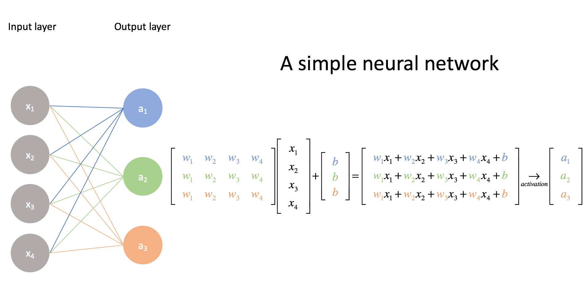
In the training of neural network models, a set of weights is established, denoted as $W$. If the neural network’s input is $x$, each layer’s output is computed by multiplying the weights with the input and applying a non-linear activation function like ReLU:
$$ h = \text{ReLU}(Wx) $$
Here, $h$ represents the model’s output.
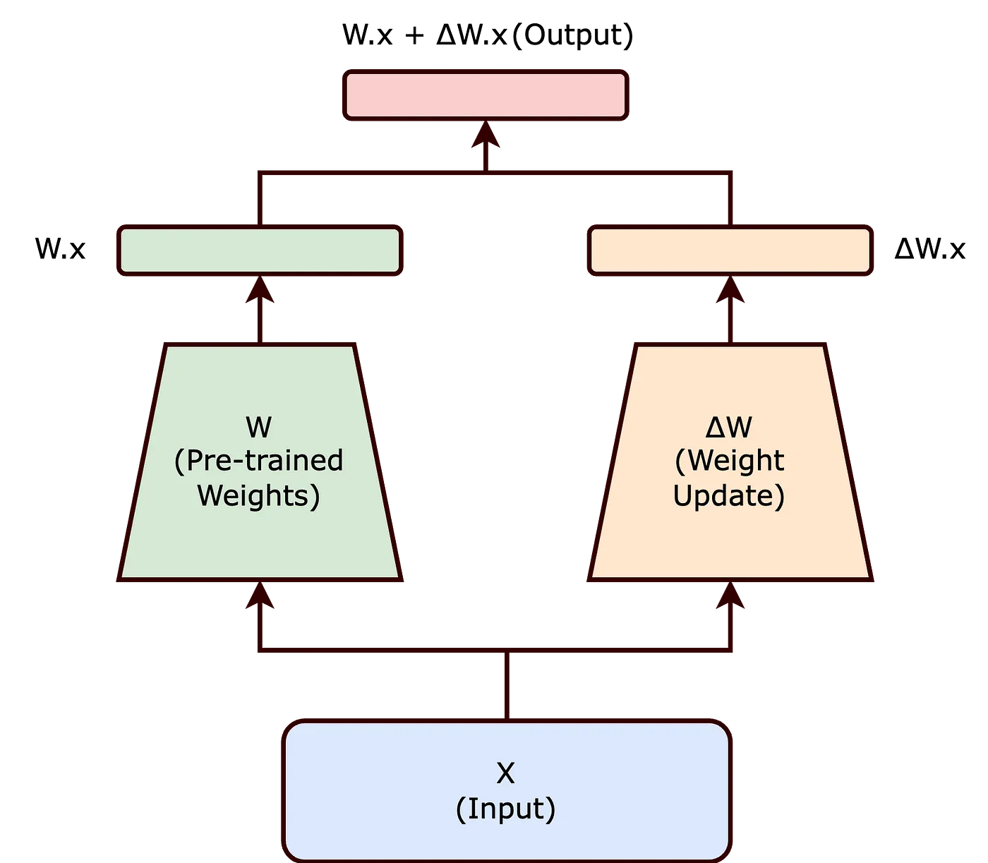
In traditional fine-tuning, the pre-trained neural network’s weights are adjusted to suit a new task. This process involves continuing training from the previous state, resulting in minor changes in the model’s weights, denoted as $\Delta{W}$, where the new model’s weights become $W + \Delta{W}$.
However, this method can be resource-intensive for Large Language Models. In LoRA, rather than directly modifying $W$, we decompose the weight matrix to achieve the desired adjustments.
The Intrinsic Rank Hypothesis #
Research suggests that the weights of neural networks are overparametrized, implying that not all weight elements are equally crucial. This idea is encapsulated in the intrinsic rank hypothesis.
The intrinsic rank hypothesis proposes that significant changes in neural networks can be captured using a lower-dimensional representation. When fine-tuning neural networks, these changes in weights can be effectively encapsulated using low-rank matrices, implying that only a subset of the weight changes is essential.
Introducing Matrices $A$ and $B$ #
Based on the intrinsic rank hypothesis, we represent $W$ with smaller matrices. Let’s assume that $W$ has dimensions $(d, k)$. We define two smaller matrices, $A$ and $B$, with dimensions $(d, r)$ and $(r, k)$ respectively.
Here, $r$ represents the rank (reduced dimension) of the matrix, serving as a hyperparameter during model fine-tuning. The number of parameters of LoRA-adapted layers depends on the value of $r$.
The product of matrices $A$ and $B$ represents the change in pre-trained weights $\Delta{W}$. Thus, the updated weight matrix ($W’$) becomes:
$$ W’ = W + BA $$
where:
$$ W’ = W + \Delta{W} = W + BA $$
$$ B \in \mathbb{R}^{d \times r}, A \in \mathbb{R}^{r \times k} $$
$$ r « \min(d, k) $$
In this equation, $W$ remains fixed (not updated during fine-tuning), while $A$ and $B$ are lower-dimensional matrices, with their product representing a low-rank approximation of $\Delta{W}$.
Authors typically initialize $A$ with random Gaussian values and $B$ with zeros, ensuring that $\Delta{W} = BA$ is zero at the beginning of training.
With LoRA, the output of the neural network becomes:
$$ h = W_0x + BAx = (W_0 + BA) x $$
Impact of Lower Rank of Trainable Parameters #
By selecting matrices $A$ and $B$ to have a lower rank $r$, the number of trainable parameters is significantly reduced.
For instance, if $W$ is a $d \times d$ matrix, traditional weight updating would involve $d^2$ parameters. However, with $B$ and $A$, the total number of parameters reduces to $2dr$, which is much smaller when $r « d$.
For example, if a model has 60,000 parameters, and the dimension of $W$ is $(300,200)$, matrices $A$ and $B$ will have dimensions $(300, r)$ and $(r, 200)$ respectively.
If $r = 4$, then the total number of trainable parameters will be $300 \times 4 + 200 \times 4 = 2000$, just 3% of the total parameters.
Similarly, if $r = 8$, then the total parameters will be 4000, still substantially lower than the original 60,000 of the model.
As models grow larger, the ratio of trainable to frozen parameters diminishes rapidly. For example, the base GPT-2 (L) model has 774 million trainable parameters, whereas the LoRA-adapted model has only 770 thousand — fewer than 0.1% of the base total.
One of the most impressive aspects of LoRA is that fine-tuned LoRA models typically perform as well as or better than their base model counterparts that have been finetuned.
The reduction in the number of trainable parameters achieved through Low-Rank Adaptation (LoRA) offers several significant benefits, particularly when fine-tuning large-scale neural networks:
- Reduced Memory Footprint: LoRA decreases memory needs by lowering the number of parameters to update, aiding in the management of large-scale models.
- Faster Training and Adaptation: By simplifying computational demands, LoRA accelerates the training and fine-tuning of large models for new tasks.
- Feasibility for Smaller Hardware: LoRA’s lower parameter count enables the fine-tuning of substantial models on less powerful hardware, like modest GPUs or CPUs.
- Scaling to Larger Models: LoRA facilitates the expansion of AI models without a corresponding increase in computational resources, making the management of growing model sizes more practical.
Implementation from Scratch using Python #
Now, Let’s implement the LORA method from scratch. You need to have basic knowledge of pytorch to understand the code.
At first, Let’s import all the required libraries
import copy

from tqdm import tqdm

import torch
import torch.nn as nn
import torchvision.datasets as datasets
import torchvision.transforms as transforms
Here, we import copy to copy our model without changing the original model.
All other libraries are from pytorch.
Next, for deterministic results, let’s set seed to some number , I will use it as 0
_ = torch.manual_seed(0)
Now let’s define a function to get the device name.
def get_device():
    if torch.cuda.is_available():
        return torch.device("cuda")
    elif torch.backends.mps.is_available():
        return torch.device("mps")
    return torch.device("cpu")
We wil use MNIST dataset, for that we download MNIST dataset and create a dataloader.
transform = transforms.Compose([transforms.ToTensor(), transforms.Normalize((0.1301, ), (0.3081, ))])

mnist_trainset = datasets.MNIST(root = "./data", train = True, download=True, transform=transform)

train_loader = torch.utils.data.DataLoader(mnist_trainset, batch_size=10, shuffle=True)

mnist_testset = datasets.MNIST(root = "./data", train=False, download=True, transform=transform)
test_loader = torch.utils.data.DataLoader(mnist_testset, batch_size=10)

device = get_device()
Let’s define a simple neural network to classify the digits.
class DigitsNet(nn.Module):
    def __init__(self, input_shape, num_classes):
        super(DigitsNet, self).__init__()
        self.linear1 = nn.Linear(input_shape, 256)
        self.linear2 = nn.Linear(256, 128)
        self.linear3 = nn.Linear(128,num_classes)
        self.relu = nn.ReLU()

    def forward(self, x):
        x = self.linear1(x)
        x = self.linear2(x)
        x = self.linear3(x)
        x = self.relu(x)
        return x
model = DigitsNet(28*28, 10).to(device)
Then, we create a function to train and test the model using the dataset we downloaded earlier.
def train(train_loader, model, epochs = 5, limit=None):
    ce_loss = nn.CrossEntropyLoss()
    optimizer = torch.optim.Adam(model.parameters(), lr=0.001)

    total_iterations = 0
    for epoch in range(epochs):
        model.train()
        loss_sum = 0
        num_iterations = 0
        data_iterator = tqdm(train_loader, desc=f"Epoch {epoch+1}")

        if limit is not None:
            data_iterator.total = limit

        for data in data_iterator:
            num_iterations += 1
            total_iterations += 1
            x, y = data
            x = x.to(device)
            y = y.to(device)

            optimizer.zero_grad()
            output = model(x.view(-1, 28*28))
            loss = ce_loss(output, y)
            loss_sum += loss
            avg_loss = loss_sum / num_iterations
            data_iterator.set_postfix(loss=avg_loss.item())
            loss.backward()
            optimizer.step()

            if limit is not None and total_iterations >= limit:
                return

train(train_loader, model, epochs=1)
OUTPUT:
Epoch 1: 100%|██████████| 6000/6000 [00:47<00:00, 125.35it/s, loss=0.72]
Let’t test the results.
def test(model):
    correct = 0
    total = 0
    wrong_counts = [0 for i in range(10)]

    with torch.no_grad():
        for data in tqdm(test_loader, desc="Testing"):
            x, y = data
            x = x.to(device)
            y = y.to(device)
            output= model(x.view(-1, 28*28))
            for idx, i in enumerate(output):
                if torch.argmax(i) == y[idx]:
                    correct += 1
                else:
                    wrong_counts[y[idx]] += 1
                total+=1
        print(f"Accuracy: {round(correct/total, 3) * 100}")
        for i in range(len(wrong_counts)):
            print(f"Wrong counts for the digit {i}: {wrong_counts[i]}")

test(model)
Testing: 100%|██████████| 1000/1000 [00:06<00:00, 156.93it/s]
Accuracy: 89.1
Wrong counts for the digit 0: 33
Wrong counts for the digit 1: 12
Wrong counts for the digit 2: 147
Wrong counts for the digit 3: 115
Wrong counts for the digit 4: 69
Wrong counts for the digit 5: 196
Wrong counts for the digit 6: 98
Wrong counts for the digit 7: 91
Wrong counts for the digit 8: 185
Wrong counts for the digit 9: 148
Here, you can see the accuracy of model is 89.1%. We can see model is performing badly in case of digits 2, 3, 5, 8 and 9. While finetuning, we finetune the model for these digits.
Now, We will create another copy of model so that we can check our output later when we finetune the model.
original_model =copy.deepcopy(model)
Before applying, Lora, let’s create a function to get the number of trainable parameters in model.
def count_parameters(model):
    return sum(p.numel() for p in model.parameters() if p.requires_grad)
count_parameters(model)

#  235,146
We have total of 235,146 parameters. Remember this number, we will compare it in later phase.
Method 1: Using Parametrization #
Let’s create a LORA Adapter which we will apply in the model. For simplicity I am using rank=1 and alpha = 1.
class LoraAdapter(nn.Module):
    def __init__(self, features_in, features_out, rank=1, alpha=1, device="mps"):
        # features_out : k, features_in: d, weight (d,k) -> (out_features, in_fecatures)
        super(LoraAdapter, self).__init__()
        self.A = nn.Parameter(torch.zeros((rank, features_out)).to(device))
        self.B = nn.Parameter(torch.zeros((features_in, rank)).to(device))

        nn.init.normal_(self.A, mean=0, std=1) # gaussian random init

        self.scale = alpha / rank
        self.enabled = True

    def forward(self, original_weights):
        if self.enabled:
            return original_weights + torch.matmul(self.B, self.A).view(original_weights.shape) * self.scale
        else:
            return original_weights
Now, I would like to discuss two methods from which we can finetune the model. There is a class parametrize, which helps us in replacing the original weights of any pytorch model. We will first go through this method. Since, this method will help us in getting the results of old model without much hassle.
So basically, parametrization replaces the parameters of model with some other function, Here in this case, we replace the “weight” of each layer with our custom function. After registering parametrization, whenever we call this layer, it will return the function we used, not the original weights of model. This will be helpful here since we don’t want to touch the original weights of model.
import torch.nn.utils.parametrize as parametrize

for name, layer in model.named_children():
    if isinstance(layer, nn.Linear):
        parametrize.register_parametrization(layer, "weight", LoraAdapter(layer.in_features, layer.out_features, rank=2, alpha=1))
Now, remember the model layers after we use parametrization, it adds additional parametrized layer in the model.
print(model)
DigitsNet(
  (linear1): ParametrizedLinear(
    in_features=784, out_features=256, bias=True
    (parametrizations): ModuleDict(
      (weight): ParametrizationList(
        (0): LoraAdapter()
      )
    )
  )
  (linear2): ParametrizedLinear(
    in_features=256, out_features=128, bias=True
    (parametrizations): ModuleDict(
      (weight): ParametrizationList(
        (0): LoraAdapter()
      )
    )
  )
  (linear3): ParametrizedLinear(
    in_features=128, out_features=10, bias=True
    (parametrizations): ModuleDict(
      (weight): ParametrizationList(
        (0): LoraAdapter()
      )
    )
  )
  (relu): ReLU()
)
Here we can see the model has Parametrized layer with LoraAdapter . Now since we are only going to train the A and B, weight matrices, we will freeze all the weights of model.
for name, param in model.named_parameters():
    if "A" not in name and "B" not in name:
        param.requires_grad = False

count_parameters(model)
# 3124
Now see, how the number of parameter decreased from 238270 to 3124. Let’s see the percentage of parameters we are going to train.
count_parameters(model)/count_parameters(original_model) * 100
# 1.32
So, we are only training 1.32% of original model. This is still a bit high number since our model is really small. For big models, This number will be in the range of 0-1.
Now, Let’s create finetuning dataset. For that, we will only use digits in which the model performed poor. We then train the model for 200 iterations. I am limiting the number of iterations for simplicity.
mnist_dataset = datasets.MNIST(root="./data", train=True, download = True, transform=transform)

for digit in [2,3,5,8,9]:
    if digit == 2:
        exclude_indices = mnist_dataset.targets == digit
    else:
        indices = mnist_dataset.targets == digit
        exclude_indices = exclude_indices | indices


mnist_dataset.data = mnist_dataset.data[exclude_indices]
mnist_dataset.targets = mnist_dataset.targets[exclude_indices]

train_loader = torch.utils.data.DataLoader(mnist_dataset, batch_size=10, shuffle=True)

train(train_loader, model, epochs=1, limit=200)
Epoch 1: 100%|█████████▉| 199/200 [00:01<00:00, 101.99it/s, loss=0.329]
Here you can see the loss is decreased from 0.72 to 0.32. But the model may have overfitted the data to only the digits we finetuned. Nevertheless, let’s see the results below.
As I said earlier, using parametrization, we will have an option to enable or disable paremetrization any time. we will create a function to do the same.
def enable_disable_lora(enabled=True):
    for layer in [model.linear1, model.linear2, model.linear3]:
        layer.parametrizations["weight"][0].enabled = enabled
Let’s check the results before finetuning.
enable_disable_lora(False)
test(model)
Testing: 100%|██████████| 1000/1000 [00:05<00:00, 171.80it/s]
Accuracy: 89.1
Wrong counts for the digit 0: 33
Wrong counts for the digit 1: 12
Wrong counts for the digit 2: 147
Wrong counts for the digit 3: 115
Wrong counts for the digit 4: 69
Wrong counts for the digit 5: 196
Wrong counts for the digit 6: 98
Wrong counts for the digit 7: 91
Wrong counts for the digit 8: 185
Wrong counts for the digit 9: 148
Now, After finetuning
enable_disable_lora(True)
test(model)
Testing: 100%|██████████| 1000/1000 [00:07<00:00, 136.35it/s]
Accuracy: 68.30000000000001
Wrong counts for the digit 0: 543
Wrong counts for the digit 1: 484
Wrong counts for the digit 2: 79
Wrong counts for the digit 3: 101
Wrong counts for the digit 4: 609
Wrong counts for the digit 5: 98
Wrong counts for the digit 6: 348
Wrong counts for the digit 7: 765
Wrong counts for the digit 8: 103
Wrong counts for the digit 9: 44
As you can see the model is performing much better for the digits we finetuned, but as suspected the model has overfitted the data. So you have to be careful when finetuning any models.
Method 2: Without parametrization #
Let’s copy the original model so that we can modify it and finetune it.
lora_model = copy.deepcopy(original_model)
Let’s create a LoraLayer This layer performs the LORA calculations and returns the changed weights.
class LoraLayer(nn.Module):
    def __init__(self, features_in, features_out, rank=2, alpha=1, device="mps"):
        # features_out : k, features_in: d, weight (d,k) -> (out_features, in_features)
        super(LoraLayer, self).__init__()
        self.A = nn.Parameter(torch.zeros((features_in, rank)).to(device))
        self.B = nn.Parameter(torch.zeros((rank, features_out)).to(device))

        nn.init.normal_(self.A, mean=0, std=1) # gaussian random init

        self.scale = alpha / rank

    def forward(self, x):
        return torch.matmul(x, torch.matmul(self.A, self.B)) * self.scale
As now we need to apply LORA layer to all of our linear layers in model and then add the weight with the original weights when inference, we create another model with all of that. I am using rank=2 here. To check how rank impacts in finetuning.
class LinearwithLORA(nn.Module):
    def __init__(self, layer, rank=2, alpha=1):
        super(LinearwithLORA, self).__init__()
        self.layer = layer
        self.lora = LoraLayer(layer.in_features, layer.out_features, rank=rank, alpha=alpha)

    def forward(self, x):
        return self.layer(x) + self.lora(x)
This layers simply adds the lora weights and original weights to get the results.
Let’s assign each of our linear layers the lora adapter.
for name, layer in lora_model.named_children():
    if isinstance(layer, nn.Linear):
        setattr(lora_model, name, LinearwithLORA(layer))
After replacing Linear layers with LoraLayer we will have the following model:
DigitsNet(
  (linear1): LinearwithLORA(
    (layer): Linear(in_features=784, out_features=256, bias=True)
    (lora): LoraLayer()
  )
  (linear2): LinearwithLORA(
    (layer): Linear(in_features=256, out_features=128, bias=True)
    (lora): LoraLayer()
  )
  (linear3): LinearwithLORA(
    (layer): Linear(in_features=128, out_features=10, bias=True)
    (lora): LoraLayer()
  )
  (relu): ReLU()
)
Here we can see our linear model is replaced by LinearwithLORA.
Let’s freeze all the previous parameters of original model so that we only train the new parameters.
for layer in lora_model.children():
    if isinstance(layer, LinearwithLORA):
        layer.layer.weight.requires_grad = False
Let’s see the number of parameters now:
count_parameters(lora_model) # 3518

count_parameters(lora_model) / count_parameters(original_model) * 100
# 1.49 %
As we increased the rank of A and B to 2, the parameters also increased by certain amount.
Now Let’s finetune the model in the same dataset we used earlier.
train(train_loader, lora_model, epochs=1, limit=200)
Epoch 1: 100%|█████████▉| 199/200 [00:02<00:00, 84.53it/s, loss=0.413]
And finally, let’s see the results.
test(lora_model)
Testing: 100%|██████████| 1000/1000 [00:07<00:00, 138.74it/s]
Accuracy: 78.0
Wrong counts for the digit 0: 88
Wrong counts for the digit 1: 503
Wrong counts for the digit 2: 97
Wrong counts for the digit 3: 101
Wrong counts for the digit 4: 361
Wrong counts for the digit 5: 119
Wrong counts for the digit 6: 120
Wrong counts for the digit 7: 651
Wrong counts for the digit 8: 103
Wrong counts for the digit 9: 55
As we can see, it did perform better than the previous method. This is due to the rank. we used rank 2 matrix here. While finetuning any models, you need to find the best value of rank and use that.
As with previous method, this method also overfitted the data, but the accuracy has improved by 10% which is huge.